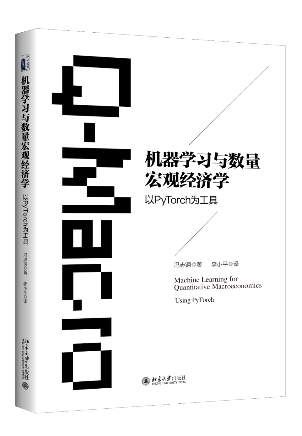
Table of Contents

Course Description and Learning Objectives

Quick Links:

• Course Materials – Lecture slides and Jupyter notebooks
• Course Recordings – Video lectures on Bilibili
• Instructor's Homepage – Additional resources

Summary

This course prepares economists to thrive in the AI era by fundamentally rethinking the researcher's role: from coder to Research Architect. The central premise is that as AI increasingly handles code implementation, the economist's competitive advantage lies in critical validation and economic safeguarding—the ability to design algorithms, direct AI tools strategically, and rigorously audit outputs for both technical correctness and economic sensibility.

Students will master computational and statistical tools for analyzing structural economic models, integrating traditional methods (dynamic programming, perturbation, projection) with modern AI/ML techniques (deep learning, reinforcement learning). The course emphasizes high-performance computing technologies and uses Python/PyTorch as primary implementation languages. Beyond technical skills, students will explore AI's broader implications for economics, including natural language processing and large language models, with content adapting to reflect the field's rapid evolution.

🎯 Learning Objectives

This course serves as a catalyst for faculty and graduate students to enhance their quantitative research capabilities. Upon completion, you will be able to:

• Analyze complex structural economic models and design appropriate solution algorithms independent of implementation tools
• Strategically direct AI coding assistants to implement computational methods efficiently, while maintaining full control over the research logic
• Apply modern computational techniques—including ML, deep learning, and reinforcement learning—to high-dimensional dynamic economic problems
• Leverage HPC technologies (JAX, distributed computing, GPUs) through both direct implementation and AI-assisted development
• Most importantly: Rigorously validate computational outputs by auditing code for technical correctness and safeguarding results against economic implausibility
• Critically evaluate AI advancements (LLMs, automated reasoning) and their implications for the future of economic research

In short: You will learn to architect research in the AI era—combining irreplaceable economic judgment with powerful computational tools, while never ceding the critical validation role that defines rigorous scholarship.

This curriculum has been continuously developed and refined since 2019 through teaching experiences at Zhongnan University of Economics and Law (2021-2024), University of International Business and Economics (2023-2025), Huazhong University of Science and Technology (2019), Iowa State University (2025), University of Miami (2025), and Wuhan University (2024, 2025).

▲ Return to Table of Contents

Course Materials

Lecture Slides

Jupyter Notebooks (Labs)

Note: Jupyter notebooks can be viewed directly on GitHub or downloaded and run locally with Python/Anaconda.

▲ Return to Table of Contents

🏛️ Hands-On Philosophy: Practicing the "Research Architect"

The hands-on sessions are the core component of this course, designed to train you in the "Research Architect" role. In the AI era, your value is not in writing boilerplate code but in your ability to specify, direct, and validate complex computational tasks. Our sessions are built around this "specification-driven" workflow.

This workflow transforms how we move from economic theory to computational results. Each hands-on exercise, from a simple cake-eating problem to a complex heterogeneous-agent model, follows this structure:

1. Mathematical & Economic Formulation:

   We start on paper, defining the optimization problem, recursive formulation (e.g., Bellman equation), and economic constraints.

2. Algorithmic Specification:

   We design a clear algorithm and write detailed pseudocode (e.g., Value Function Iteration, Euler-equation-based solver). This is the "human logic" that cannot be outsourced.

3. Define Deliverables:

   We explicitly state our goals. What outputs do we need? A plot of the policy function? A graph showing Euler equation errors? A table of simulated statistics exported to a file?

4. AI-Augmented Implementation:

   We feed this precise specification (Steps 1-3) to an AI assistant (like ChatGPT, Claude, or Copilot) to generate the initial Python/PyTorch code.

5. Critical Validation & Expansion:

   This is the most crucial step. We audit the AI's output for technical bugs, economic plausibility, and numerical stability. We then refine the algorithm, expand the model, or enhance the analysis, starting the loop over.

This approach differs fundamentally from static, pre-AI notebooks. The implementation is live, customizable, and expandable. You are in an interactive loop with the AI—using it to fill knowledge gaps (e.g., "Explain this PyTorch function") while you simultaneously safeguard the output with your economic and computational judgment.

These sessions are designed to prove a critical point: your background understanding matters. We will tackle problems where a vague prompt yields a flawed or simple-minded AI response. You will see how providing more detailed, economically-informed instructions and rigorous validation (i.e., being a good Research Architect) allows you to produce more robust, accurate, and sophisticated results.

▲ Return to Table of Contents

List of Topics

(Subject to change based on field advancements and class interest)

Topic 1: Artificial Intelligence for Economics Research

Conceptual Content

• The Paradigm Shift: From Coder to Research Architect
  • Four competencies: Theoretical Mastery, Technical Fluency, AI-Augmented Implementation, Critical Validation.
• Evolution of AI: Foundations (1950s) → Deep Learning (2010s) → Generative Era (2017–Present).
• Key Technologies: Machine learning, deep learning, NLP, and LLMs.
• Two Pillars: Economics of AI vs. AI for Economics.
• Soft vs. Hard Analysis: AI excels at synthesis; humans remain essential for novel proofs and economic judgment.
• Applications: Big data, forecasting, causal inference, solving DSGE models, text analysis.

Topic 2: Introduction to Computation for Macroeconomists

Conceptual Content

• What is Quantitative Macroeconomics?
  • Using numerical methods and computational tools to solve and analyze macroeconomic models.
  • Core methods: dynamic programming, numerical optimization, Monte Carlo simulation.
• Workhorse Models in Quantitative Macro:
  • Neoclassical (stochastic) optimal growth model.
  • Bewley-Aiyagari-Huggett model (incomplete markets).
  • Krusell-Smith model (aggregate uncertainty).
  • Overlapping generations (OLG) models.
  • New Keynesian DSGE models.
• Theoretical Foundations for Computing the Optimal Growth Model:
  • Principle of optimality and recursive formulation.
  • Contraction mapping theorem and Blackwell's sufficient conditions.
  • Theorem of the maximum and dynamic programming.
  • Euler equations and recursive equilibrium.
• Numerical Techniques Required:
  • Function approximation and interpolation (splines, Chebyshev polynomials).
  • Numerical optimization and differentiation.
  • Stochastic process approximation (Tauchen, Rouwenhorst).
  • Linearization, perturbation, and projection methods.
  • Machine learning techniques (DNNs, reinforcement learning).
  • Grid construction and adaptation.
• Programming Languages: Python, PyTorch, and the Anaconda ecosystem.

Topic 3: Programming Basics for Economists

Conceptual Content

• Introduction to Python and PyTorch:
  • Key programming concepts for numerical and AI applications.
  • Variables and Data Types: integers, floats, strings, booleans, lists, dictionaries, tuples.
  • Basic Operations: arithmetic, logical, comparison, and string operations.
  • Functions and Classes:
    • Defining functions, parameters, return values, and scope.
    • Object-oriented programming basics: classes, methods, inheritance.
    • Lambda functions and functional programming concepts.
  • Control Structures: if-else statements, for/while loops, list comprehensions.
  • Modules and Packages: importing, creating custom modules, virtual environments.
  • Exception handling and debugging strategies.
• NumPy fundamentals:
  • Array creation, indexing, slicing, and broadcasting.
  • Vectorized operations and performance benefits.
  • Linear algebra operations with numpy.linalg.
• Setting up and running machine learning code with ChatGPT or similar AI tools:
  • Best practices for AI-assisted coding.
  • Code review and validation techniques.

Topic 4: Numerical Methods for Macroeconomists

Conceptual Content

• Introduction to numerical methods:
  • Function approximation: polynomial, spline, and piecewise methods.
  • Numerical optimization: gradient-based and derivative-free methods.
  • Root-finding algorithms: bisection, Newton-Raphson, secant method.
  • Interpolation: linear, cubic spline, and shape-preserving methods.
  • Numerical differentiation: forward, backward, and central differences.
  • Numerical integration: quadrature methods (Gaussian, Simpson's rule).
• AR(1) Approximation and Numerical Simulation:
  • Discretization methods: Tauchen, Rouwenhorst methods.
  • Simulation techniques and ergodic distributions.
  • Statistical properties of discretized processes.
• Practical examples and implementation in Python:
  • Using scipy.optimize, scipy.interpolate, and numpy.
• Applications to basic economic models:
  • Consumer optimization problems.
  • Firm production decisions under uncertainty.

Topic 5: Introduction to Machine Learning for Economists

Conceptual Content

• PyTorch for Economists:
  • Tensors, computational graphs, and automatic differentiation (autograd).
  • Building neural networks with torch.nn.
  • Training loops and optimizers (SGD, Adam, RMSprop, etc.).
  • Using tqdm for progress tracking and performance monitoring.
  • Distributed Data Parallelism (DDP) in PyTorch: Scaling up training for large models or datasets.
  • Device management: CPU vs. GPU computation.
• Deep Learning Basics:
  • Neural network architecture: layers, neurons, and connectivity.
  • Activation functions: ReLU, Sigmoid, Tanh, and their properties.
  • Loss functions: MSE, Cross-Entropy, and custom losses.
  • Gradient descent and backpropagation mechanics.
  • Overfitting, regularization (L1, L2, Dropout), early stopping, and validation strategies.
  • Batch normalization and other normalization techniques.
• Economics-Focused Extensions:
  • Custom loss functions to incorporate economic constraints (utility, equilibrium conditions, monotonicity).
  • Handling panel data or time series with PyTorch.
  • GPU/parallel processing for large-scale economic models.
  • Interpreting neural network predictions in economic contexts.

Topic 6: Solving Macroeconomic Models Using Machine Learning

Conceptual Content

• Value Function-Based Approaches:
  • Deep Neural Network (DNN) Approximation: Representing value and policy functions with neural nets.
  • Value Function Iteration (VFI) under the DNN framework.
  • Introduction to the Actor-Critic algorithm for dynamic optimization.
  • Monte Carlo simulation for policy evaluation.
  • Temporal-Difference (TD) learning in value approximation.
• Euler Equation-Based Approaches:
  • Reformulating the problem as a supervised learning task.
  • Leveraging PyTorch for function approximation and gradient-based methods.
  • Residual minimization techniques.
  • Time iteration vs. policy iteration in neural network context.
• Implementation Tips:
  • Structuring Python/PyTorch code for dynamic models (modularity, reusability).
  • Debugging and performance profiling in large-scale simulations.
  • Parallelization (DDP) and GPU utilization for faster training.
  • Convergence diagnostics and error metrics.
• Comparison with traditional methods:
  • Accuracy, speed, and scalability trade-offs.
  • When to use ML vs. classical methods.

Topic 7: Numerical Solution Methods for Dynamic Models

Conceptual Content

• Numerical solutions of dynamic equilibrium models:
  • Discrete-time dynamic programming fundamentals.
  • Bellman equations and the principle of optimality.
  • Contraction mapping theorem: existence, uniqueness, and convergence rate.
  • State space discretization and approximation theory.
• Value function iteration (VFI):
  • Algorithm implementation and convergence criteria.
  • Grid construction: uniform, logarithmic, Chebyshev nodes.
  • Interpolation schemes: linear, cubic spline, shape-preserving.
• Euler equation-based methods (time iteration):
  • Deriving Euler equations from first-order conditions.
  • Fixed-point iteration on policy functions.
  • Convergence properties and comparison with VFI.

Topic 8: Advanced Numerical Methods and Accuracy Assessment

Conceptual Content

• Acceleration techniques:
  • Howard's policy improvement algorithm.
  • MacQueen-Porteus bounds.
  • Exploiting monotonicity and concavity in policy functions.
• Endogenous Grid Method (EGM):
  • Inverting the Euler equation to avoid root-finding.
  • Computational gains and extensions.
• Accuracy assessment:
  • Euler equation errors: construction and interpretation.
  • Den Haan-Marcet statistics.
  • Convergence diagnostics and method comparison.

Topic 9: Perturbation and Projection Methods

Conceptual Content

• Perturbation methods:
  • Euler Equation-Based Methods and deterministic steady states.
  • Expanding around steady states: Taylor series approximation.
  • First-order (linear) and second-order approximations.
  • Blanchard-Kahn conditions for saddle-path stability.
  • Pruning schemes for higher-order approximations.
  • Advantages and limitations: accuracy vs. speed, local vs. global.
• Projection methods:
  • Global approximation techniques: spectral and finite element methods.
  • The choices of basis functions: polynomials, wavelets, splines.
  • Chebyshev polynomials and orthogonal projection.
  • Smolyak's algorithm for high-dimensional approximation (curse of dimensionality mitigation).
  • Finite element methods: piecewise approximation and adaptivity.
  • Determining coefficients for basis functions: collocation, least-squares, Galerkin.
  • Choosing appropriate weight functions and residual functions.
  • Tensor product grids vs. sparse grids.
• Practical applications in macroeconomic modeling:
  • When to use perturbation vs. projection vs. global methods.
  • Hybrid approaches combining multiple techniques.

Topic 10: High-Performance and Parallel Computing (HPC)

Conceptual Content

• Serial vs. Parallel computing:
  • Benefits: Time reduction, cost efficiency, and scalability.
  • Challenges: Communication overhead, load balancing, debugging complexity.
• Applications in Economics:
  • Climate-economy models (e.g., Cai and Lontzek 2019).
  • Large-scale heterogeneous agent models.
  • Monte Carlo simulations and policy analysis.
• Core Concepts:
  • HPC architecture: clusters, nodes, and resource management.
  • CPU, cores, and threads: understanding hardware.
  • Shared vs. Distributed memory models.
  • Amdahl's Law and the limits of parallelization.
  • Speedup, efficiency, and strong/weak scaling.
• Parallel Programming with MPI (Message Passing Interface):
  • Master/worker paradigm and task distribution.
  • Basic operations: MPI_Init, MPI_Finalize, MPI_Comm_rank, MPI_Comm_size.
  • Point-to-point communication: MPI_Send, MPI_Recv.
  • Collective communications: MPI_Gather, MPI_Scatter, MPI_Bcast, MPI_Reduce.
  • mpi4py for Python-based MPI programming.
• Parallel Computing in PyTorch:
  • Using the GPU: .to(device) and tensor operations.
  • Data Parallelism: nn.DataParallel (single machine, multi-GPU).
  • Distributed Data Parallelism: nn.DistributedDataParallel (DDP) for multi-node training.
  • Best practices for efficient GPU utilization.
  • Profiling and optimization techniques.
• Working with HPC clusters:
  • SLURM job scheduler: submitting jobs, resource allocation, monitoring.
  • Module systems and environment management.
  • Job arrays and parameter sweeps.

Topic 11: Heterogeneous Agents Models with Machine Learning

UPDATED 2026Slide deck: Lec_2026_11_ML_HA_models.pdf

Conceptual Content

• Foundations in Aiyagari–Bewley–Huggett:
  • Stationary Recursive Competitive Equilibrium (SRCE) and market clearing.
  • Existence/uniqueness of invariant distributions (Feller, mixing, monotonicity conditions).
  • Economic interpretation of precautionary savings and wealth inequality.
• Canonical computational pipeline:
  • For a fixed interest rate, solve household policy functions.
  • Compute stationary distributions from the induced transition kernel.
  • Update prices until excess demand for capital is near zero.
• Global solution with deep learning and RL ideas:
  • Actor-critic style updates for value and policy networks.
  • Distribution-aware state representation and simulation-based training.
  • Transition from stationary equilibrium analysis to full distributional dynamics.
• Krusell-Smith with modern ML methods:
  • DeepHAM: two-network setup (value + policy), Monte Carlo simulation, and fictitious-play updates.
  • DEQN: Euler-equation-based method with a single policy network and cloud simulation across many economies.
  • DeepHAM vs. DEQN trade-off: richer distribution representation vs. simpler Euler-residual training.

Topic 12: Heterogeneous-Agent OLG Models (Classic & ML Methods)

Conceptual Content

• The Challenge:
  • Life-cycle features: finite horizon, age-dependent policies.
  • Inter-generational heterogeneity: cohorts with different characteristics.
  • Intra-generational heterogeneity: idiosyncratic shocks within cohorts.
• Part 1: Classic Methods (Idiosyncratic Shocks Only)
  • Stationary Recursive Competitive Equilibrium (SRCE) definition.
  • Algorithm: Nested fixed point (outer loop on prices, inner loop on VFI and distribution).
  • Backward induction: solving for optimal policies by age.
  • Distribution computation via transition matrix method (forward iteration).
  • Bilinear interpolation for off-grid points.
  • Market clearing conditions: capital, labor, and goods markets.
  • Deterministic transition dynamics: backward-forward iteration.
  • Tax and transfer system modeling.
• Part 2: ML Methods (Aggregate Shocks)
  • The challenge: distribution as a high-dimensional state variable.
  • Neural network approximation with a "market clearing layer".
  • Endogenous price determination within the network.
  • Training via minimizing Euler residuals and market clearing errors.
  • Fisher-Burmeister complementarity function for non-negativity constraints.
  • Stabilizing homotopy techniques:
    • Capital-only models as initialization.
    • Price pre-training for stability.
    • Gradual introduction of government bonds.
  • Handling lifecycle dimension with age-specific networks or conditioning.

Topic 13: Asset Pricing with Machine Learning

Conceptual Content

• Foundations of Asset Pricing:
  • Stochastic Discount Factors (SDF) and Arrow-Debreu securities.
  • The Consumption-CAPM (C-CAPM) and the Lucas Tree model.
  • The Equity Premium Puzzle: Why standard utility functions fail to match historical data.
• The Empirical Pivot:
  • Linear Factor Models: From Fama-French (3 factors) to the "Factor Zoo" (300+ factors).
  • The curse of dimensionality in empirical finance.
• Machine Learning Solutions (The GKX Framework):
  • Treating asset pricing as a non-parametric prediction problem ($r_{t+1} = g(z_t) + \epsilon$).
  • The Gu, Kelly, and Xiu (2020) approach: Using Neural Networks to capture non-linearities and interactions.
  • Universal Approximation: Why Deep Learning outperforms OLS and Lasso in return prediction.
• Performance Evaluation:
  • Out-of-sample $R^2$ metrics for financial data.
  • Constructing efficient frontiers and analyzing Sharpe Ratios of ML-driven portfolios.

Topic 14: Reinforcement Learning

Conceptual Content

• Reinforcement Learning (RL) for Economics:
  • Framework for sequential decision-making under uncertainty.
  • Natural fit for dynamic optimization and control problems.
  • Agent, environment, state, action, reward structure.
• Markov Decision Processes (MDPs):
  • Formal framework: states, actions, transition probabilities, rewards.
  • Policies, value functions, and optimal policies.
  • Bellman optimality equations.
• From MDPs to Monte Carlo and Temporal-Difference (TD) Methods:
  • Value function estimation with episodic (Monte Carlo) updates.
  • Incremental (TD) updates: TD(0), TD(λ).
  • Exploration–exploitation trade-offs and ε-greedy policies.
  • On-policy vs. off-policy learning (SARSA vs. Q-learning).
  • Ensuring learning stability and convergence.
• Function Approximation and Deep RL:
  • Neural networks for high-dimensional value and policy functions.
  • Deep Q-Networks (DQN) and experience replay.
  • Policy gradient methods: REINFORCE, advantage estimation.
  • Actor-critic architectures for continuous state/action spaces.
  • Proximal Policy Optimization (PPO) and Trust Region methods.
  • Deterministic Policy Gradient (DPG) and DDPG.
• RL in Economic Applications:
  • Optimal taxation and fiscal policy.
  • Monetary policy design.
  • Portfolio management and trading strategies.
  • Market design and mechanism design.

Topic 15: Mean Field Games (MFG) in Continuous Time

Conceptual Content

• Motivation:
  • Heterogeneous agents and the "curse of dimensionality".
  • Mean field approximation: representing aggregate behavior.
  • Applications in economics: large populations, anonymous interactions.
• The Core MFG Feedback Loop:
  • Individual optimization given mean field (distribution of others).
  • Aggregate behavior determines the mean field.
  • Consistency condition: individual optimization → aggregate behavior → mean field.
• The Engine Room: A Tale of Two Equations:
  • Hamilton-Jacobi-Bellman (HJB): Individual optimization problem (solves backward in time).
  • Kolmogorov Forward Equation (KFE): Distribution evolution (solves forward in time).
  • Coupled system: policy from HJB affects drift in KFE, distribution from KFE affects HJB.
• Numerical Solution for HJB:
  • The Upwind Scheme: finite difference method for handling controlled drift.
  • Choosing between forward and backward differences based on drift direction.
  • Stability and convergence properties.
• The MFG System and Duality:
  • Relationship between HJB and KFE operators: AT (matrix transpose).
  • Variational formulation and optimality conditions.
• Algorithm for Stationary Equilibrium:
  • Iterating on HJB (given distribution), KFE (given policy), and prices.
  • Fixed-point iteration and convergence criteria.
• Transition Dynamics:
  • The backward-forward shooting algorithm.
  • Solving for equilibrium paths between steady states.
  • Boundary conditions and terminal conditions.
• Applications in Economics:
  • Dynamic models of income and wealth inequality.
  • Optimal taxation in large populations.
  • Financial markets with heterogeneous traders.

Topic 16: Large Language Models

Conceptual Content

• Introduction to LLMs:
  • Relevance of text analysis in economics: policy documents, corporate filings, news, social media.
  • Key concepts: Transformer architecture basics, autoregressive generation.
  • Evolution: from Word2Vec to BERT to GPT to modern LLMs.
• Representing Text Numerically:
  • Tokenization strategies: word-level, subword (BPE, WordPiece), character-level.
  • Vocabulary construction and out-of-vocabulary handling.
  • Word embeddings: TF-IDF, Word2Vec, GloVe—mechanisms and economic applications.
  • Applications: Economic Policy Uncertainty (EPU) index, inflation forecasting, gender norms in language.
  • Positional encodings for sequence awareness (sinusoidal, learned).
• The Transformer Architecture:
  • Core mechanism: Self-attention (Queries, Keys, Values).
  • Multi-head attention: parallel attention mechanisms.
  • Scaled dot-product attention and computational efficiency.
  • Supporting components: feed-forward networks, residual connections, layer normalization.
  • Encoder-decoder vs. decoder-only architectures.
  • Comparison: advantages over static embeddings and topic models (LDA, NMF).
• LLMs in Practice:
  • Model scale and examples: GPT series, BERT, T5, LLaMA.
  • Text generation process: greedy decoding, beam search, sampling strategies.
  • Training: pre-training fundamentals (self-supervised learning on large corpora).
  • Fine-tuning for domain-specific tasks: classification, named entity recognition, question answering.
  • Prompt engineering and in-context learning.
  • Reinforcement learning from human feedback (RLHF).
• LLMs in Economics Research:
  • Applications:
    • Advanced sentiment/policy analysis: central bank communications, FOMC minutes.
    • Innovation measurement: analyzing patents and R&D documents.
    • Forecasting enhancements: incorporating textual data.
    • Event studies: measuring market reactions to news.
  • Integrating LLM outputs (e.g., sentiment scores, text features) into economic models.
  • Causal inference with textual instruments.
  • Limitations and challenges: bias, interpretability, computational cost.

References

• Judd, Kenneth. Numerical Method in Economics.
• Ljungqvist, Lars, and Thomas J. Sargent. Recursive Macroeconomic Theory.
• Goodfellow, Ian, Yoshua Bengio, and Aaron Courville. Deep Learning.
• Bertsekas, Dimitri. Reinforcement Learning and Optimal Control.
• Feng, Zhigang. Machine Learning for Quantitative Macro.
• Santos, Manuel S. Numerical Solution of Dynamic Economic Models.
• QuantEcon Lectures (https://quantecon.org/lectures/)

Acknowledgments

▲ Return to Table of Contents